On this page, we show how fit data to the power exponential function (PowExp, Elashoff et al, 1982), and we compare the results with those of the LinExp-fit.

# gastempt3.r
# (C) 2005 Dieter Menne, http://www.menne-biomed.de
# Comparing Power Exponential fits with LinExp Fits
# PB: Pinheiro/Bates, Mixed-Effect..., Springer 2000
library(nlme)    # Mixed effect number crunching
library(lattice) # Trellis plots
options(digits=3) # print 3 significant digits
# Get our standard functions from external file in same folder
source("fitfuncs.r")

# Get Data from comma-separated (csv) file with header
ge = read.table("gastempt.csv",sep=",",header=TRUE)
# Make sure subject are not treated as numbers
ge$subj = as.factor(ge$subj)
# Create new factor <subj>.<treat>
ge$subjtreat = as.factor(paste(ge$subj,ge$treat,sep="."))
Nothing new till here. In the source-in file fitfuncs.r we have defined the function SSEmptPowExp as a self-starting power exponential function. Wenn running it with nlsList, we get a series of error messages.
gePowlist = nlsList(v~SSEmptPowExp(t,v0,beta,tempt)|subjtreat,data=ge)
Error in qr(attr(rhs, "gradient")) : NA/NaN/Inf in foreign function call (arg 1)
In addition: Warning message: NaNs produced in: log(x)
The approximation fails because the coefficients cannot be constrained to positive value in the current implementation, and negative coefficients give undefined logarithms when the gradient is computed.
As a workaround, we estimate the logarithm of the coefficients. If required, after all nls/nlme calculations we can convert the log-coefficients back to base values. This is similar to the phenobarbital example in PB, chapter 6.4. To stay consistent, we also estimate the logarithms of the coefficients for the LinExp case, even if this is not strictly required. The self-starting functions SSEmptPowExpLog and SSEmptLinExpLog are defined in fitfuncs.r.
gePowLoglist = nlsList(v~SSEmptPowExpLog(t,v0,logbeta,logtempt)|subjtreat,data=ge)
geLinLoglist = nlsList(v~SSEmptLinExpLog(t,v0,logkappa,logtempt)|subjtreat,data=ge)
print(gePowLoglist)
print(geLinLoglist)
Coefficients:
         v0 logbeta logtempt
10.alb  581  -0.329     5.31
10.lip  632   1.743     4.55
11.alb 1103  -0.349     5.94
11.lip  861   1.314     4.81
12.alb  547   1.265     4.76
12.lip  703   1.255     4.54
2.alb   436   0.570     5.35
2.lip   779   1.109     4.55

Degrees of freedom: 88 total; 64 residual
Residual standard error: 31.0
There is no NA in the PowExp fit, all single fits converged, but the LinExp fit gave the well know two non-converging cases (details not show here). The standard residual error was 31 for PowExp and 26 for LinExp, indicating a somewhat better fit for the latter. This comparison is flawed because of the NA in LinExp, but we will confirm the general finding below.
# compute nlme fits
# PowExp fit
contr = nlmeControl(pnlsTol=0.3)
ge3PowLog.nlme=nlme(gePowLoglist,control=contr)
ge3PowLog.coef = coef(ge3PowLog.nlme)
print(ge3PowLog.nlme)
print(ge3PowLog.coef)
Nonlinear mixed-effects model fit by maximum likelihood
  Model: v ~ SSEmptPowExpLog(t, v0, logbeta, logtempt)
...
Residual  31.6
...
The logarithm (base e=2.7...) of the fitted parameters
         v0 logbeta logtempt
10.alb  518  0.3616     5.01
10.lip  636  1.5236     4.57
11.alb 1068 -0.0833     5.64
We have a residual variance of 31.6 for the PowExp fit, which we can compare with the variance of the LinExp fit of 28.7 below. The reduction in residual error with LinExp is not very strong, and it should not be used as the sole criterion to prefer one model over the other. The main argument in favor of LinExp is a qualitative one, namely that it can model the initial overshoot with the same number of parameters as the power exponential model.
# LinExp fit

ge3LinLog.nlme=nlme(geLinLoglist,control=contr)
ge3LinLog.coef = coef(ge3LinLog.nlme)
print(ge3LinLog.nlme)
print(ge3LinLog.coef)
Nonlinear mixed-effects model fit by maximum likelihood
  Model: v ~ SSEmptLinExpLog(t, v0, logkappa, logtempt)
...
Residual  28.7
...
The logarithm (base e=2.7...) of the fitted parameters
         v0 logkappa logtempt
10.alb  532   -0.154     4.29
10.lip  550    0.710     3.78
11.alb 1065   -0.769     5.05
...
If required, logkappa and logtempt could be converted kappa and tempt with kappa = exp(logkappa) for tabulation. However, to compute predictions we better continue to use the logs.
# Compute t50
ge3LinLog.coef$t50 = apply(ge3LinLog.coef,1,t50)
ge3PowLog.coef$t50 = apply(ge3PowLog.coef,1,t50)
The function t50 which computes the 50% emptying times is programmed to handle both PowExp and LinExp and their logarithms in an intelligent way, so we don't have to call different functions for the four cases.
# Find maximum of all t50 for plotting range
t50.max = floor((max(c(ge3LinLog.coef$t50,ge3PowLog.coef$t50))*1.2)/10)*10

# Using "augmented prediction", this time with extrapolation
ge3LinLog.pred = augPred(ge3LinLog.nlme,primary=~t,maximum=t50.max)
levels(ge3LinLog.pred$.type) = c("predlin","original")
ge3PowLog.pred = augPred(ge3PowLog.nlme,primary=~t,maximum=t50.max)
levels(ge3PowLog.pred$.type) = c("predpow","original")
ge3.pred = rbind(ge3LinLog.pred,
                 ge3PowLog.pred[ge3PowLog.pred$.type == "predpow",])
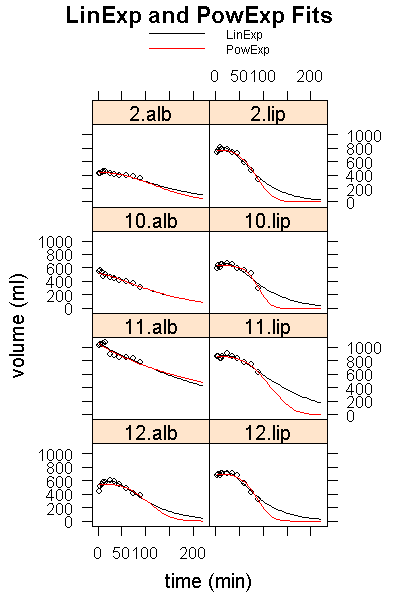
Function augPred is a powerful tool from the nlme toolbox. For a given model, it computes a data frame that contains all the original data points and nicely spaced model-predicted data points together. When we plot augPred data, we get data and fit overlaid to easily check the quality of the model.
The lines below could be abbreviated as plot(ge3.pred) in interactive R-mode, everything else is only decorative.
# prepare a few trellis settings to unclutter plot
par.settings = list(plot.symbol = list(col="black",cex=0.5),
          superpose.line = list(col=c("black","blue","red"),
                                lty=1))
key =  list(lines = list(col=c("black","red")),
         text=list(lab=c("LinExp","PowExp"),cex = c(0.6)))

p = plot(ge3.pred,
        layout=c(2,4), aspect=0.7,as.table=T,
        main="LinExp and PowExp Fits",
        xlab="time (min)", ylab="volume (ml)",
        par.settings = par.settings, key=key)
print(p)

Click here for a pdf version of the graph where you can better see the details in the initial parts of the curves. By definition, the PowExp function cannot follow the initial bump if it is present, but the deviations are not very large. More seriously, however, PowExp falls off very quickly for curves with a large overshoot, possibly giving too low estimates of half-emptying times for these curve forms.
# Output the plot to a postscript file
trellis.device("postscript",file="gastempt3.ps",
  theme="col.whitebg",horizontal=F)
print(p)
dev.off() # don't forget to close the device
# Diagnostic plots of residuals
# remove two # for png output
#trellis.device("png",file="gastempt3_diag%03d.png",
#  width=400,height=600,theme="col.whitebg")
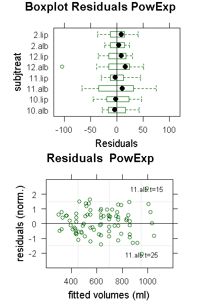
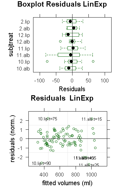
Looking at the original data and fits produces by augPred is nice, but for a detailed diagnostic we should check the residuals, i.e. the signed deviations of the data from fits, normalized to the standard deviation. R can mark outliers, so rechecking bad readings should be easy.
PlotResids = function(nlmefit,title) {
  p = plot(nlmefit,subjtreat ~resid(.), abline = 0,
     main= paste("Boxplot Residuals",title),aspect=0.7,
     xlim=c(-120,120))
  print(p,split=c(1,1,1,2),more=TRUE)

  print(p,split=c(1,1,1,2),more=TRUE)
  p = plot(nlmefit,
    id=0.05,  # mark significant deviations
    idLabels = paste(ge$subjtreat,ge$t,sep=".t="), # add time
    main =  paste("Residuals ",title),
    ylab = "residuals (norm.)",
    xlab = "fitted volumes (ml)",
    aspect=0.7, cex=0.7,xlim=c(200,1200),ylim = c(-3,3)
    )
  print(p,split=c(1,2,1,2))
}

PlotResids(ge3PowLog.nlme,"PowExp")
PlotResids(ge3LinLog.nlme,"LinExp")


In the residuals plot we can see that for subject 11, albumin the values at t=15 and t=25 are outliers in opposing directions. Closer inspection of the data reveals that between these two the curve shifted, so it is probably not a bad reading, but some systematic shift we cannot do anything against. There are more outliers in LinExp compared to PowExp; note that the deviations are normalized to the standard deviation which is smaller for LinExp as for PowExp, so LinExp fits are more sensitive to outliers because of the better fit.
#dev.off() # remove first # for png output
And don't forget to close your device when you write to some external file, otherwise the last plot will be lost.

 Dr. Dieter Menne
 07072 1263 688
