Multiple indexing with Stan
January 15, 2020, 8:00 pmSummary
Using vectors for indexed access to ragged arrays in Stan
volume ~ normal(
      v0[record] .* (1+ kappa[record] .* (minute ./ tempt[record])) .*
      exp(-minute ./ tempt[record]), sigma);
Fitting gastric emptying time series
Gastric volume times serie measured by MRI techniques can have an initial volume overshoot due to secretion. To estimate half-times and the degree of overshoot, the author of this blog has introduced the linexp function [@Fruehauf2011] with three parameters to complement the power exponential function used in earlier research [@Elashoff1982, @Elashoff1983b] with scintigraphic data.
linexp:
v = v0* (1+t*kappa/tempt)*exp(-t/t_{empt})In mathematical notation:
\(v = v0(1+\frac{t\cdot\kappa}{t_{empt}})e^{-t/t_{empt}}\)
Fitting individual curves with the linexp model can result in extreme results because of a strong correlation between kappa and tempt at values of kappa < 0.7. When the fit is not reliable, R function nls laconically waves goodbye with greetings from Douglas Bates, yet GraphPad and Matlab give answers against better knowledge. In case you should take the coefficients from individually fitted curves seriously, check their standard errors.
The R package gastempt has some tools to generate simulated gastric emptying data and to fit the linexp and power exponential function using nonlinear mixed models with package nlme. By analyzing whole studies instead of individual curves, one can tap the power of "borrowing strength" and obtain much more reasonable descriptors of gastric emptying curves.
Here is a set of simulated data and the fit computed with nlme:
Get Simulated Data
library(gastempt)
library(ggplot2)
library(rstan)
library(stringr)
rstan_options(auto_write = TRUE)

# Install package dmenne/gastempt if it is not yet available
if (!require("gastempt")) {
  # Get model
  devtools::install_github("dmenne/gastempt")
}
# Generate sample data with 15% missing (from package gastempt)
d = simulate_gastempt(n_records = 6, missing = 0.35,
                      max_minute = 180, # Use short records
                      student_t_df = 3, # generate outliers
                      kappa_mean = 1.2, seed = 212)
# Compute fit using nlme and wrapper nlme_gastempt in package gastempt;
fit_d = nlme_gastempt(d$data)
Function nlme_gastempt is a wrapper around nlme and also returns a ggplot graph of data and fitted curves.
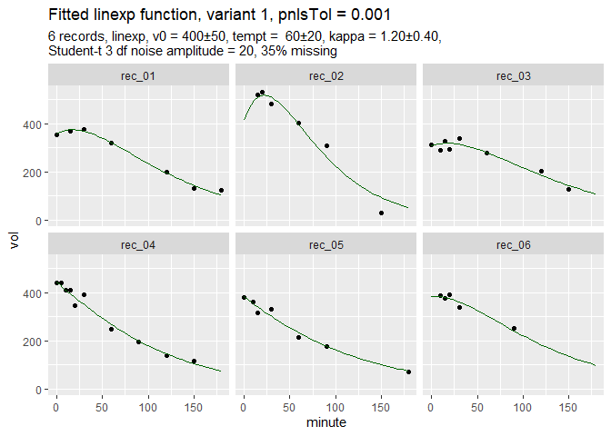
The simulated data are dirty and incomplete by design to show the power of the population fit. In more extreme cases, nlme might fail, but Stan can do the job, slowly but safely.
Run Stan
# Get model from package gastempt and run Stan
chains = 1
iter  = 10000L # For easier benchmarking. fewer iterations ok
# NOTE: Compiling the model needs several minutes
run_stan = function(model, data)  {
  model_file  = paste0(model, ".stan")
  # Keep Stan quiet (it is very verbose even with verbose = FALSE)
  cap = capture.output({
    mr =  suppressWarnings(
      stan(model_file, data = data, chains = chains, iter = iter,
               seed = 4711)
      )
  })
  list(mr = mr, model_file = model_file)
}
The number of iterations (iter = 10000) is higher than required for convergence to reduce dependency on overhead for benchmarking.
Conventional indexing with loop
m_1b = run_stan("linexp_gastro_1b", d$stan_data)Full Stan code for this model is available here, and is precompiled in package gastempt. This code uses indexing in a loop which has been supported since the first versions of Stan:
for (i in 1:n){
   reci = record[i];
   v0r = v0[reci];
   kappar = kappa[reci];
   temptr = tempt[reci];
   vol[i] = v0r*(1+kappar*minute[i]/temptr)*exp(-minute[i]/temptr);
  }
  volume ~ normal(vol, sigma);
}
Multiple indexing with vectors
With more recent versions, vectorized indexing can be used (Stan reference 2.10, Section 5) which should give more efficient code. Here the relevant part of the code:
m_1c = run_stan("linexp_gastro_1c", d$stan_data)The Stan source code for this model can be found here. The core model line looks like this:
volume ~ normal(vol, sigma);Note that .* is used for elementwise vector multiplication; no loop is required.
Multiple indexing with manual subexpression evaluation
In the above example, the subexpression minute ./ tempt[record]) is computed twice. Is the compiler clever enough to optimize this, or should we tweak manually?
m_1d = run_stan("linexp_gastro_1d", d$stan_data)Full Stan code for this model. The subexpression can be computed in the transformed parameters section.
transformed parameters {
  vector[n] mt;
  mt = minute ./ tempt[record]; // manual optimization
}

model{
volume ~ normal(vol, sigma);
}And the winner is...
stan::get_elapsed_time was used to get the time for 10000 iterations and 1 chain.
| model | warmup | sample | total | reltime |
|---|---|---|---|---|
| Loop | 2.34 | 2.68 | 5.02 | 1.00 |
| Multiple indexing | 2.97 | 3.74 | 6.71 | 1.34 |
| Multiple indexing + optimization | 2.68 | 3.06 | 5.74 | 1.14 |
- Multiple indexing is slower :-( .
- Manual subexpression optimization does not pay.
- Maybe I did not get the right form yet?